(Pelevina et al., 2016) at Proc. RL-NLP

Mmm, word sense plus graph theory. I’m in heaven. This paper proposes a way to determine word senses (is that band the bracelet or band the musical group) from normal embeddings using clustering and ego networks. Their results are comparable to the state of the art. Unfortunately, the state of the art doesn’t beat the majority-class heuristic.

The big problem in word vectors is different meanings. This can manifest itself as homography: two words spelled the same way, like wind and wind, as well as polysemy: related meanings like bank as a building or a financial institution. Sussing these apart is the task of “word sense disambiguation”. (You can also take a harder task: determining the number of senses out of thin air, word sense induction.)

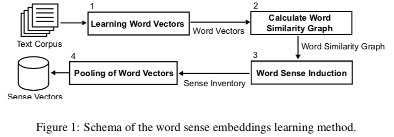
The authors use a rather straightforward pipeline.

1. Learn word vectors from text.
2. Calculate a graph of word similarity from the vectors
3. Perform word sense induction: get an inventory of senses
4. Pool the word vectors into sense vectors

There are a million strategies for learning word vectors. (I personally like the idea of linguistically motivated sparse vectors if you have the data in your language.)

Once you have those, you can compute cosine similarity between vectors. With such a large space, this is time-consuming. The authors do block matrix operations, with block-size 1000. The authors used a threshold of 200—each node was connected to its 200 nearest neighbors. (Could we have devised a variable number of connections instead of KNN?)

With our graph in place, we construct ego graphs for each word. An ego graph is every node within some number of hops of the source node, e.g., everyone I can reach in two hops or fewer. Everyone in the ego graph is then connected to their n most similar words. Finally, we cluster using the Chinese Whispers algorithm. (Shockingly, this is equivalent to the label propagation algorithm? Nobody caught on?) LPA is great because it makes no assumption about the number of clusters. (That’s also true of other community detection algorithms, though.)

The authors’ choice of LPA is disappointing because it produces different results on each run, so generally people take a consensus among multiple runs. Or they just use a different algorithm. Still, those results are demonstrably better on average than, say, the leading eigenvector algorithm—which is consistent from run to run.

To compute the sense inventory from the produced clusters, they took the average (weighted or unweighted) over the vectors in each cluster. Weight, if used, were the similarities of each word to the word whose senses we want to uncover.

Finally, with an inventory of senses in hand for each word, we must disambiguate. We have two choices for how to do this. One is to maximize the probability of the context given the sense—basically CBOW word2vec. \(\mathbf{\overline{c}}_c\) is the mean context embedding of the context words.

\[s^* = \arg\max_i P(C \mid \mathbf{s}_i) = \arg\max_i \frac{1}{1 + e^{-\mathbf{\overline{c}}_c \cdot \mathbf{s}_i}}\]

The other choice is to maximize the similarity between the sense and the context. This time, we take the mean of the word embeddings of the context words.

\[s^* = \arg\max_i \mathit{sim}\left(\mathbf{s}_i, C\right) = \arg\max_i \frac{\mathbf{\overline{c}}_w \cdot \mathbf{s}_i}{\mid\mid\mathbf{\overline{c}}_w\mid\mid \cdot \mid\mid\mathbf{s}_i\mid\mid }\]

As a last trick, they compute the discriminative power of each word, taking only the \(p\) most discriminative for their model. Their score function is either of the two functions we argmaxed above.

\[\max_i \mathit{score}(\mathbf{s}_i, c_j) - \min_i \mathit{score}(\mathbf{s}_i, c_j)\]

Evaluation

They play with their model on a dataset of thousands of annotated sentences for about 1000 nouns, “with an average polysemy of 2.26 senses per word”. Each noun has an explicit sense, given by a list of synonyms. As is true of normal word use, the dataset is skewed toward one dominant sense per word. The authors test both this and a class-balanced version, so that just guessing the dominant sense doesn’t win you anything.

They also note that another method just used k-means clustering on the contexts, instead of their graph-based model. Unfortunate in that approach is the need to specify your k.