(Malaviya, Gormley, and Neubig, 2018) at ACL (to appear)

Good morphological taggers (the software that sees hablaste and recognizes that it’s in the preterite tense, second-person singular) are important because they’re used to improve later tasks. Today’s paper presents a state-of-the-art neural tagger based on neural nets and conditional random fields. I’d previously looked at combining neural nets and graphical models, and I think this is a better example.

Morphological tagging involves taking a sequence of words and marking the properties of those words. It’s similar to part-of-speech tagging, except that the tags aren’t atomic, like NOUN or ADJ. Instead, they’re sets of individual features, like {POS: Adj, Gender: Masc, Number: Sing}. If your schema defines \(\mid \mathcal{S} \mid\) features, each word could be tagged with one of \(2^{\mid \mathcal{S} \mid}\) bundles. Malaviya et al. make a simplifying assumption: words will never have two tags from one category. For instance, Gender can only be one of Masc, Fem, Neu, or <Not relevant>, not some combination.

The authors work with the Universal Dependencies treebank, a collection of running text that’s annotated with morphological bundles. Because UD is compiled by different annotators, the categories applied to the same word can be different from language to language. This inconsistency has weakened previous taggers, which assume that the space of bundles will match between the languages. The probability of the tag sequence given the sentence is:

\[\Pr(\mathbf{y} \mid \mathbf{x}) = \prod_{t=1}^T \Pr(\mathbf{y}_t \mid \mathbf{x})\]

Malaviya et al. break from past work by individually predicting each feature in the bundle—instead of the entire bundle as a unit. Instead of regarding tagging as a multi-class problem, they treat it as multi-label classification. If each label were independent, we could get the conditional likelihood as:

\[\Pr(\mathbf{y} \mid \mathbf{x}) = \prod_{t=1}^T \prod_{m=1}^M \Pr(y_{t,m} \mid \mathbf{x})\]

That’s not to say that they predict features independently. Instead, they model relationships between features in a bundle, along with sequential relationships, using a conditional random field. This is a globally normalized model which can define arbitrary dependencies, scored according to a chosen potential function \(\psi\).

\[\Pr(\mathbf{y} \mid \mathbf{x}) = \frac{1}{Z(\mathbf{x})} \prod_{t=1}^T \prod_{\alpha \in \mathcal{C}} \phi_\alpha(\mathbf{y}_\alpha, \mathbf{x}, t)\]

Z is the normalizing constant for this sentence, ensuring that the probability distribution is valid. Each alpha is an individual factor, one of the colored boxes in the figure. The factor touches some circles representing variables, which we call \(\mathbf{y}_\alpha\).

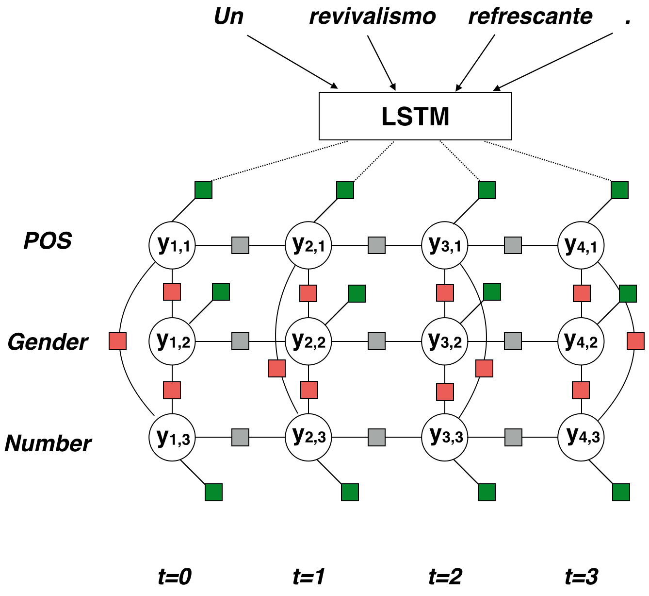
In this case, the green potentials are calculated using an LSTM.

1. Create word vectors. Run a character-level bi-LSTM over each word. This gives a forward sequence and backward sequence of hidden states. Take the last states of each sequence and concatenate them to get the word embedding. We do this to include subword information in the word embeddings.
2. Process the sentence. Now, we use a word-level bi-LSTM. It takes the word embeddings as input and produces two sequences of hidden states, just like step 1. This time, we concatenate the two vectors for each word, making our word representations aware of their context.
3. Use a language-specific linear layer \(\mathbf{g}(\mathbf{x}, t \mid \ell) = \mathbf{W}\ell\mathbf{e}_t + \mathbf{b}\ell\) to transform each word vector into a score vector. There’s one entry for each of the \(M\) categories.
4. Take a linear combination of the scores, then exponentiate it—which ensures that the result is positive. This is your potential value. (Potentials must be positive.)

The red pairwise potentials and grey transition potentials are also exponentiated linear combinations, though there’s no nonlinearity involved. An innovation for these is that they share general linguistic knowledge: Learned weights \(\lambda\) are a sum \(\lambda_{\rm general} +\lambda_{\rm language}\).

To actually perform inference with this loopy-graph model, they resort to loopy belief propagation, a message-passing algorithm. Variables (circles) and factors (squares) take turns computing messages and propagating them to their neighbors, in an arbitrary order. After the messages converge (the error is below some threshold), you can compute the final values at each position as a function of the messages. Those values are, more or less, probabilities which can be used or inference.

At test time, they decode using minimum Bayes risk, maximizing the probabilities for each tag. Their loss is Hamming loss (lose a point for every true/false you have to flip).

Little tricks to make it work:

• The final task is to improve tagging by exploiting a high-resource language (HRL). Unfortunately, both their model and the baseline overfit the HRL, so they upsample the low-resource text by a factor of 10.
• Comparing Adam and SGD as optimizers.

They actually wind up smoking the baseline by Cotterell and Heigold. The idea that the individual features should be related is unsurprising. What’s cool about this paper is how they made it work.