(Dyer et al., 2015) at ACL and IJCNLP

Today’s paper tackles a method for putting a continuous representation inside of a dependency parser.

Ah, beautiful shift-reduce parsing. This simple method (with a small lookahead) is a bit of magic that has been behind compilers for years. It’s a quaint, constant-time technique which has only two actions to perform for each input token—when the grammar is unambiguous, as it must be for a programming language. Natural language is different; do the same tricks work when ambiguity abounds?

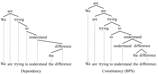
Let’s first review dependency parsing. Unlike the constituency parsing that you’re familiar with from middle school English classes which use a phrase structure grammar, or constituency grammar (noun, verb phrase, etc.), a dependency grammar has exactly one node in the parse tree for each word. (It can actually have one per morph, if you choose to break words into sub-word units.) Each node points to exactly one parent called a head, on which it depends. (The exception is the ROOT node, which isn’t shown below. It’s assumed that the sentence’s head points to ROOT.)

---

Today’s paper relies on three stack LSTMs, the authors’ custom data structure which can both push and pop inputs—they can read or forget, in the LSTM sense of ‘forget’. So let’s review how LSTMs work and build up to these stack LSTMs.

LSTMs are a specialized RNN. An RNN maintains an internal (‘hidden’) state which is used to compute outputs. It is also updated as the RNN observes each next part of a sequential input. The new hidden state \(\mathbf{h}_t\) is a function (a 1-layer MLP) of the previous hidden state \(\mathbf{h}_{t-1}\) and the input \(\mathbf{x}_t\). It’s easy for this MLP’s sigmoidal activation to dampen the importance of long-term effects over time, because you repeatedly squash the old value.

LSTMs introduce a memory ‘cell’ to combat this. The values in the cell are a sum of the input and ‘forget’ values—though ‘forget’ should probably be called ‘remember’. The values for each are a 1-layer sigmoidal MLP drawing values from the input, the previous hidden state, and the previous cell state. The sigmoid squeezes each into the range (0, 1). The new cell value is then some fraction of the previous cell value, plus some learned function of the input and hidden state, squeezed to (-1, 1). Now, we can update the hidden state as a sigmoidal function of the cell state, previous hidden state, and input.

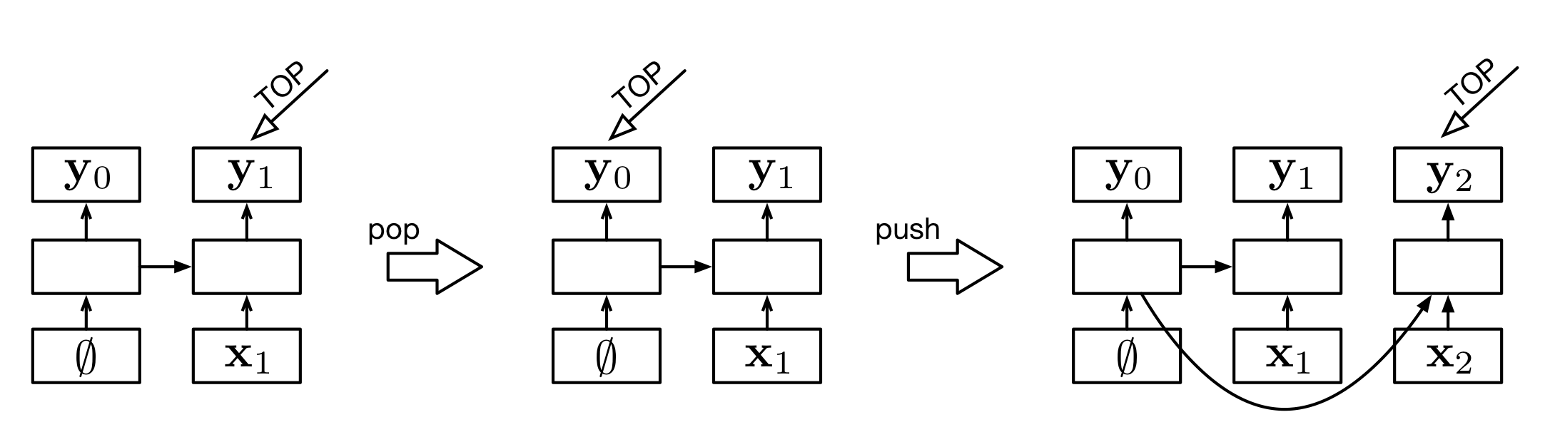
The stack LSTM adds a ‘stack pointer’, which is completely similar to the stack pointer in programming languages. (That is, a state is a combination of the hidden state, cell state, and stack pointer—a back pointer!) Instead of using the immediately previous cell and hidden states, the pointer points back through history to select one. New inputs are pushed on the right, as normal. The pop operation amounts to moving the pointer to the previous element. Contents are never overwritten in this LSTM.

Do you really need to keep the hidden everything, instead of just overwriting? Yes: Even though the new parts aren’t part of the stack, they still produce outputs. The fact that we keep everything, including back pointers, lets the stack represent a tree. Convince yourself below.

---

We’ll work with three stacks: a buffer \(B\) of unprocessed words, a stack \(S\) of the partial parse, and \(A\), the action history—I’ve seen this called a trace. Tokens move from the buffer to the stack, or tokens from the stack are popped and merged. Each one of these actions is recorded in the trace.

To determine the state of the parser after an action, they use a 1-layer ReLU net which takes the encodings of the current stack, buffer, and trace. Each of the possible actions has an embedding and bias which are used as affine transformations of the current state \(\mathbf{p}_t\), then these are softmaxed to get the probability of a given action \(z_t\). (The softmax function is essentially “Give me a probability distribution from my vector of real numbers”.)

\[ p(z_t \mid \mathbf{p}_t) = \frac{\exp(\mathbf{g}_{z_t}^\intercal \mathbf{p}_t + q_{z_t})}{\sum_{z’ \in \mathcal{A}(S, B)} \exp(\mathbf{g}_{z’_t}^\intercal \mathbf{p}_t + q_{z’_t})} \]

You can also just treat this as a softmax layer after a different linear layer for each action. The probability of an action sequence is then expressible the same way as we do in language modeling.

To combine their embeddings in the REDUCE operations, they run linear->tanh over the head, dependent, and an embedding of the relation (the parser action). When I implemented this, I just used a one-hot (sparse) embedding because they make no claims about how the embeddings were formed.

---

As an aside, I like what they did to embed their tokens. It’s an affine+ReLU mix of pre-trained embeddings and vector representations that they learned from their own data. (Also they had POS tag data.) In each training epoch, they dropped out half of their singleton words with the unknown-word token (UNK). This sounds like it would make their model flexible to words that aren’t in their embedding vocabulary—though don’t most common words now exist in things like already-trained word2vec embeddings? Ah, they didn’t use pre-trained embeddings. They used a word2vec modification which includes positional encodings of the words.

---

As is common, the authors maximized the log-likelihood of treebank parses given sentences. Not that anyone should obsess over hyper-parameters and how they trained, but they used stochastic gradient descent (again, common) with leaning rate decay (also common) and no momentum (which is nowadays uncommon). To regularize, they applied an L2 penalty to the weights—force the weights to be small, and you’ll hopefully generalize better. They also used Glorot initialization for their weights.

Their data sources are super Stanford-y, which makes sense given that Chen and Manning of Stanford were the first to succeed at neural dependency parsing. They used the English and Chinese Gigaword corpuses (‘corpora’ bugs me) to learn their word vectors using the word2vec adaptation I mentioned earlier.

They also claim that they outperform the Chen and Manning parser in almost every setting. I’m impressed by how many papers claim excellent results like this—do papers that don’t achieve this just not get published? If so, people are making so much progress. Otherwise, maybe everyone compares to the same older baseline instead of the new state of the art. When is a result a result?

Closing thoughts

• They point out that composed tree fragments outperformed head-only representations, then suggest ‘implications for theories of headedness’—but they don’t dive into these. I haven’t bought into dependency parsing, so I’m not surprised that you need broad information.
• It’s interesting that beam search didn’t improve their results over greedy decoding. I saw the same thing in my implementation of their model.

TLDR

• Making your LSTM stack-y by building from points arbitrarily far in the history lets you encode trees, which improves performance on dependency parsing. The authors managed to make a shift-reduce parser using neural networks.