(Collins, Dasgupta, and Schapire, 2001) at NIPS

Principal component analysis was the dimensionality reduction technique we learned in my machine learning class at SMU. The start of every pipeline was center, scale, and run PCA. Unfortunately, as it’s presented, it’s designed for continuous data. This paper extends it to other data types: integers and booleans.

A review: vanilla PCA and probability

PCA is a much-loved, hundred-plus-year-old dimensionality reduction technique developed by Karl Pearson. It’s typically described as a linear projection which maximizes the variance in the projected space. Working with \(d\)-dimensional data points \(\mathbf{x}_1, \ldots, \mathbf{x}_n\), we project the data into the subspace to get \(\boldsymbol{\mu}_1, \ldots, \boldsymbol{\mu}_n\). Keeping the components with the greatest variance is expressible as minimizing the distance between the projections and the original data.

(We need to constrain the \(v\)s to be \((k < d)\)-dimensional, which I don’t express here.)

Collins et al. point out that PCA has a probabilistic interpretation. Each data point \(\mathbf{x}_i\) is taken as a random draw from a Gaussian distribution centered at \(\boldsymbol{\mu}_i\). We want to find the parameters \(\boldsymbol{\theta} = {\boldsymbol{\mu}_i}\) that maximize the likelihood of the data while still remaining in the subspace. (This aligns with one part of my color inventories model—we have ‘universal’ chromemes in space that are corrupted by Gaussian noise into particular chromes. Cotterell and Eisner (2018) also did this, but they didn’t point out that it’s PCA.) This is equivalent to our objective up above because the negative log-likelihood of a normal distribution is what we got above. Why? Let’s take a look.

The likelihood of the data in the multivariate Gaussian distribution given the means and covariance matrix \(\boldsymbol{\boldsymbol{\Sigma}}\) is easy to find on Wikipedia:

One assumption of PCA is spherical covariance—there’s no correlation between components. \(\boldsymbol{\Sigma}\) is diagonal. This simplifies our math. We wind up with a constant times the exponential of \(-\frac{1}{2}(\mathbf{x} - \boldsymbol{\mu})’(\mathbf{x} - \boldsymbol{\mu})\). That’s the expression for the dot-product, which we can express in the usual notation: \(-\frac{1}{2}\mid\mid\mathbf{x} - \boldsymbol{\mu}\mid\mid\). I mentioned the exponential earlier; when we take the negative log of that, we get \(\mid\mid\mathbf{x}_i - \boldsymbol{\mu}_i \mid\mid^2\). That’s sufficiently cool. And the constant that came from the determinant in front can be ignored, because it doesn’t depend on the data or the means. The last step is to add up all of the errors for each term, and we get the expression at the very top.

Forgetting everything we know, opening our minds

The big assumption up above is that the noise is Gaussian: Each data point is drawn from a Gaussian distribution around the ‘true’ data.

But that doesn’t have to be the case. We can use a Poisson distribution for integer data or a Bernoulli distribution for binary data. And you can also mix and match. You just need the natural parameter for each distribution (mean for Gaussian, etc.) and to maximize the log-likelihood while keeping the data in your low-dimensional subspace.

When working with data that aren’t Gaussian, the parameters and the data won’t necessarily be in the same space anymore. For instance, Bernoulli is a weighted coin-flip. The weight is a real value in \([0, 1]\), but the data can only take on two values: \({0, 1}\).

The exponential family of distributions (and some light statistical mechanics)

The exponential family is in the title, and we named some specific examples. Let’s look at the family more generally.

The function \(G\) is the log of our normalizer, or the free energy—not that the name is important. It makes the probabilities conditioned on theta add up to 1. Perhaps it’d be better to write it as \(F(\theta) \equiv \log Z(\theta)\) for that reason. In some rather widespread notational formalisms, we then get \(F(\theta) = \log \sum_{x \in \mathcal{X}} P_0(x) e^{x\theta} \). In this case, we have a very simple Hamiltonian function in the exponent: \(H(x) := \theta x\). And now we’re in the world of statistical mechanics. Let’s turn back before I introduce more hopeless notation and names.

The authors show how the likelihood functions for different exponential-family distributions match up piece-by-piece to the above equation. Each has a different closed form for it. We also care about the derivative \(F’(\theta)\), because it equals the expected value of the data given the parameters:  \(F’(\theta)=\mathbb{E}[x\mid\theta]\). (If someone asks, I’ll upload hand-written scribbles of a proof.)

An aside: generalized linear models

The authors next motivate their method by its connection to generalized linear models (GLMs), so it’s time for a Bayesian stats primer. GLMs extend linear regression, also to the exponential family of distributions. The objective function looks very similar, except that in PCA the data are unobserved, and they’re constrained to some subspace.

In linear regression, we want to fit a line through a set of points. We express this as a minimization problem: we want some parameters \(\boldsymbol{\beta}\) which minimize \(\sum_i(y_i - \boldsymbol{\beta} \cdot \mathbf{x}_i)^2\). The justification is pretty similar to up above. To generalize this, we rely on a link function, whose inverse is denoted \(h\). The link function is cool because it means that your matrices don’t need to be constrained—the function handles it for you. People love the canonical link \(h=F’\). In this case, the natural parameters \(\boldsymbol{\theta}\) are approximated by \(\boldsymbol{\beta} \cdot \mathbf{x}_i\). You can feed this into the log-likelihood up above for the exponential family.

Setup: notation

Let’s tie this back to PCA. Now, we don’t know the weights, but we also don’t know the data points. We want each \( \boldsymbol{\mu}i \) close to each \( \mathbf{x}_i \) but in a lower-dimensionality subspace. A subspace can be represented by a basis: linearly independent vectors \[\mathbf{v}_1, \ldots, {\mathbf{v}\ell} \]. Each \(\boldsymbol{\mu}i\) is then a linear combination of those basis vectors: \( \boldsymbol{\mu}_i = \sum_k a{ik} \mathbf{v}_k \).

There’s some ironing out of notation that needs to be done here to flesh out the analogy, and it’s complicated because in one case, we want to fit the \(\mathbf{x}_i\)s and in the other, we’re fitting the \(y_i\)s using the \(\mathbf{x}_i\)s. One big change to clear things up: we won’t use \(\boldsymbol{\mu}\) anymore, because it has a very Gaussian chauvinism to it—\(\boldsymbol{\mu}\) typically represents the mean of a Gaussian distribution. Instead, we’ll use the more general \(\boldsymbol{\theta}\) for whatever the distribution of interest’s natural parameter is.

So we have a matrix of data points \(\mathbf{X}\) which we want to approximate as linear combinations of basis vectors: \(\boldsymbol{\Theta} = \mathbf{A}\mathbf{V}\), i.e. a set of points in the subspace \(\mathbf{V}\). We want our approximation to represent the data well, so we maximize the posterior probability the data given the parameters. If we negate that, we get a loss function to minimize:

How do we do it?

Normally, PCA can be solved with a linear algebra technique called singular value decomposition (SVD). When treated as an optimization problem, we can perform alternating optimization, starting from a random basis and operating for t iterations:

for j in range(n): a[i][t] = argmin(a, L(V[t-1], A))
for j in range(d): v[j][t] = argmin(v, L(V, A[t]))

Each of these amounts to solving a single-variable GLM—play with the notation above and you can show it. Collins et al. show that, because of what the updates are for a Gaussian distribution, this is equivalent to SVD when we assume Gaussian PCA.

The loss isn’t convex in both arguments, which makes optimizing difficult. Otherwise, everything is linear, so we could just use linear programming. Interestingly, it’s convex in either argument when the other is held fixed. Still, we can’t guarantee convergence—except in the Gaussian case. There are a few more details (to avoid catastrophic failure of the optimization) that I won’t cover here.

Examples!

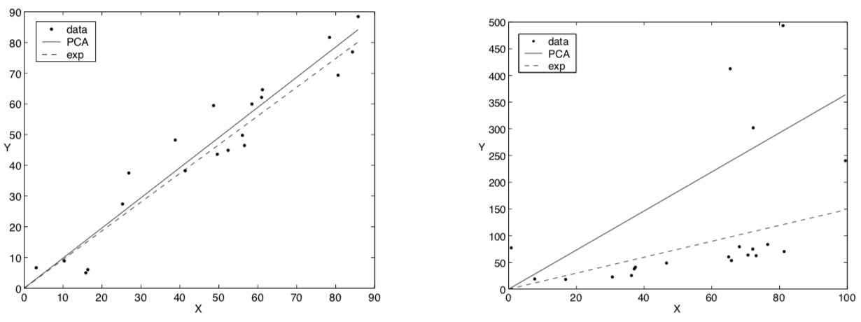
Now we’ll look at the exponential distribution, which is a member of the exponential family. Different things. Similar names. The distribution is over nonnegative real numbers. The density is usually expressed \(P(x; \alpha) = \alpha e^{-\alpha x}\), and the mean is \(\frac{1}{\alpha}\). Keeping this in the form of \(e^{\theta x}\) means \(\theta = -\alpha\). Pushing the front \(\alpha\) into the numerator, the density is now \(P(x; \theta) = e^{\theta x - G(\theta)}\) with our log-normalizer \(G(\theta) = - \log(-\theta)\). Our link function, which should approximate the mean, is \(G’(\theta) \equiv F’(\theta) = - \frac{1}{\theta}\). The authors give a closed-form update rule here, too. And they show on two toy examples that exponential PCA (which, because of its link function, must produce a line) is more resiliant to outliers.

The authors also give us a 1D projection of Bernoulli PCA, which has an eerily Ising model–like feel to it. Could you reduce the decision of some subset of a set?

Questions:

• Exponential distribution PCA also requires a line through the origin, but how do you center the data, like you would for Gaussian distributed PCA?
• How about actually reducing dimensionality on new data? The sticky wicket here is that you can get values that are in a different space. The way to do it, though, is to hold the basis \(\mathbf{V}\) fixed and optimize the weights \(\mathbf{A}\).

The bottom line: Other types of data besides continuous variables with a Gaussian assumption can be reduced to lower-dimensionality hypotheses.