SMU’s algorithm engineering class has been facetiously called a “course in computational creativity.” This creativity was stretched into graph theory for the class’s final project: fast algorithms for graph coloring and finding communication backbones in wireless sensor networks.

My implementation of the smallest-last ordering for greedy coloring was my first contribution to Python’s networkx graph library.

With the increasing prevalence of IoT devices and Bluetooth beacons, finding reliable communication pathways is becoming a critical problem. Interference, contention, and routing each become complicated problems when wireless sensors are randomly distributed. This motivates the investigation of communication backbones which can serve as trunk lines for the communication.

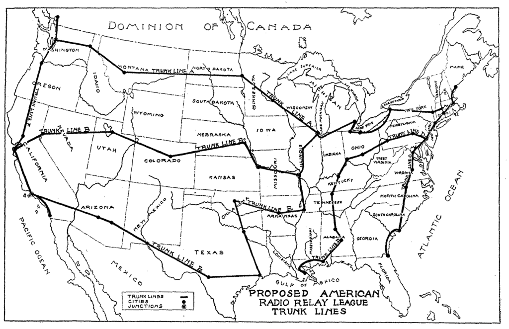Large-scale trunk lines for communicating in the USA

A model of the wireless sensor network is the random geometric graph (RGG). Nodes in the graph are connected if they are within a given radius r, which meshes with our intuitive understanding of wireless signal range. A really approachable primer on wireless sensor networks and RGGs is here.

A minimal (cheap) backbone communicates with as many nodes as possible, while including as few nodes as possible. A trick for finding the backbone is using the graph coloring—putting the nodes into as few buckets as possible, with no adjacent nodes in the same bucket. The buckets are independent sets. A single independent set in an RGG tries to cover as much of the space as possible, without letting the nodes communicate. Merging two independent sets lets them serve as relays for one another.

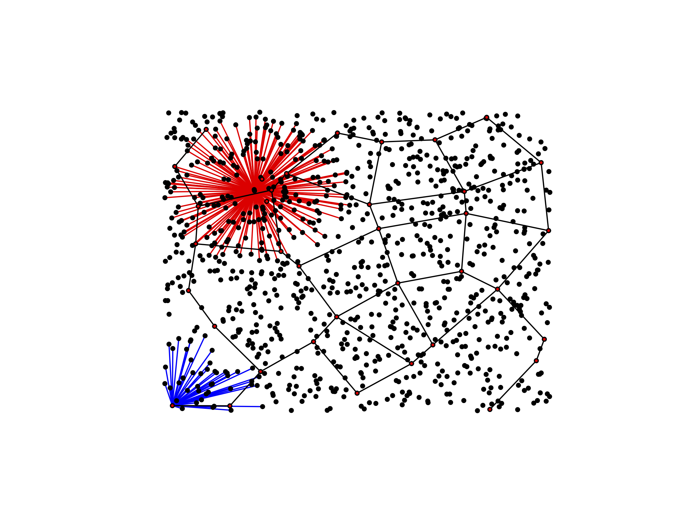Nodes marked in red form the backbone with the greatest coverage, and black edges connect the backbone. The red edges connect a single node to all of its neighbors.

While graph coloring is an NP-complete problem, numerous heuristics have been proposed. My thesis advisor, David W. Matula, presented the smallest-last ordering. It repeatedly removes a node of least degree until the graph is empty. Along the way, you wind up with a terminal clique: every node left has the same degree, because they’re all connected to one another. The graph will need at least as many colors as the terminal clique size.

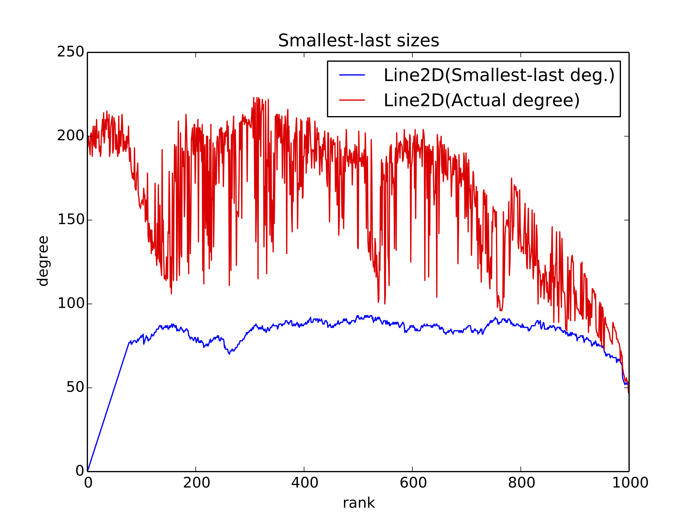The terminal clique is discernible at the far left of the graph, where the slope is consistent.

Along the way, I learned some pretty cool tricks for speeding up the implementation:

• Fast random point generation on a sphere—avoids rejection sampling (which is not guaranteed to terminate) and transcendental functions. It produces a 25% speedup over the next best method.
• k-d trees for quickly determining the edges present in a random geometric graph. It beats the O(n^2) brute-force algorithm.
• Speeding up the smallest-last ordering by using a bucket queue data structure optimized by tracking the lower bound on degree. The naive algorithm is O(n^2); this is O(n+m). I added my to networkx, so I anticipate seeing it show up in future students’ projects without attribution. Shrug.
• Computing faces on the sphere using the Euler characteristic, instead of by counting.

My full writeup for the project is here, and the code is here.